Being a previous Alteryx user, I was a little perplexed about how things worked and where things were within the EasyMorph. Where are the icons? The connectors? No macros? Tools? How does this work? Below, I put together a pretty simple, straightforward guide for "translating" Alteryx to EasyMorph. Please note, this is not a comparison piece addressing which one is "better" than the other, but rather a guide to help people coming from Alteryx, or using EasyMorph alongside Alteryx.
![]()

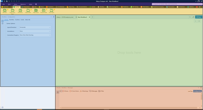
THE GUI
In the Alteryx UI, the application menu/options reside along the top (purple), with the Tool menu/”ribbon” just below (yellow). Tool settings lie along the left side (blue). The central canvas, where the workflow is constructed takes up most of the center-right (green), and the bottom (orange) is where a sample of the active dataset is displayed. The bottom-left corner, by default is open, but can display the “Overview” (top-level view) of the entire workflow if desired.
WORKFLOW COMPARISON
WORKFLOW PREMISE
Alteryx uses individual tools (each icon representing a “tool”) connected by connectors (lines and arrows) to represent the flow of data through the workflow. On the left and right sides of a tool are the anchors for connecting upstream and downstream tools. Left anchors (one or more) receive the data stream from previous tools, while the right-side anchors deliver the modified dataset to the next tools in the chain. To give the workflow a cleaner, uncluttered look in larger workflows, connectors can be made “wireless” (hidden). Each category of tools is represented by a different color: input/output = green, preparation = dark blue, joins = purple, etc.
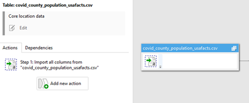
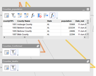
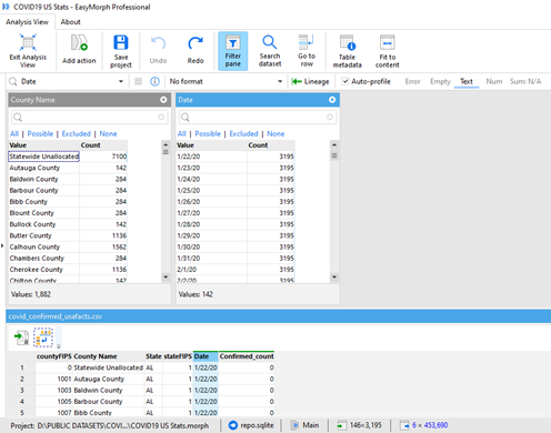
While the focal points of Alteryx’s workflow are the tools, connectors, and the workflow overall, EasyMorph’s primary focus is on datasets. Each dataset in the workflow is represented as a table, with the data showing at the bottom in a grid (this can be resized or hidden). Above the data grid, below the title bar, is the Action “row”. As actions are added to a dataset, the actions’ icons line up in order from left to right, forming the chain of actions that modify the dataset .
Datasets are connected to each other either indirectly, using join/merge actions (illustrated by a dotted line connecting the reference dataset to the join/merge action in the primary dataset), or directly, in the case of derived tables and reports (illustrated by using solid lines/arrows connecting the source dataset to the derived dataset/report).
WORKFLOW STRUCTURE
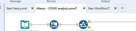
Alteryx workflow structure is pretty straightforward – a single workflow, or even separate independent workflows, can reside in a single tab. As such, each tab can be considered more of a “project” than just a workflow and is saved as its own Alteryx file. Workflows can call other workflows designed as macros (.yxmc files) – specialized workflows which receive data, process it, and can return the results back to the calling workflow. Multiple workflows (tabs) can be opened simultaneously in the UI, but each represents an individual file.
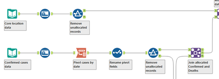
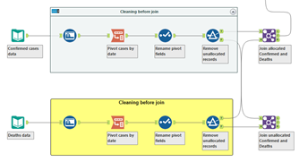
Alteryx workflows can be visually segregated into functional sections using container or comment tools, although the entire workflow still resides within a single tab. In the pic below, the top branch is contained within a container tool, while the bottom branch is contained within a comment box. Container tools can be enabled or disabled to turn “on” or “off” the sections of the workflow within them.
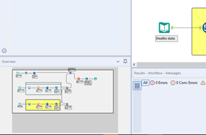
To navigate larger workflows, the Overview pane can be opened (lower-left in the UI) and manipulated to move around the workflow structure.
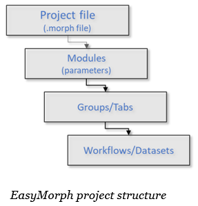
EasyMorph uses more of a “hierarchy” to define its project structure. At the top of the hierarchy is the .morph file itself, which is considered a project, or project file.
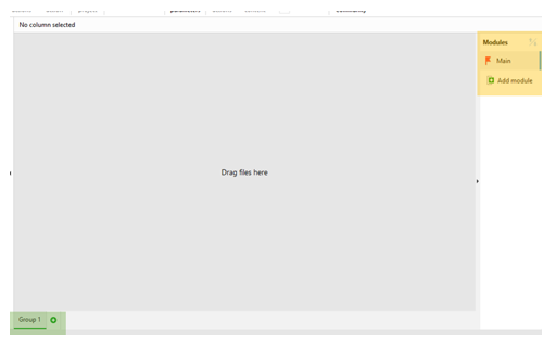
Projects contain one or more modules, which are listed in the Module pane at the right of the UI (orange in the pic below-right). A module is an independent, complete workflow with its own set of groups/tabs and parameters. A project file starts off with a default module named “Main”, although this can be renamed as the user sees fit.
Modules can be added to create “subroutines” that can be called from other modules within this project file, or from workflows residing in other project files. Modules are a great way to create reusable, standardized routines that may be utilized by multiple workflows.
One module within the workflow is set as the default module – the starting point of the workflow. By default, this is the “Main” module when the workflow is first created (but could have been renamed by the user). To assign a different module to be the starting point, right-click on the module name at the right and select “Set as default module” from the context menu.
At the next level down, each Module contains one or more tabs or groups (along the bottom of the UI; green in the pic above-right). Groups are where the actual workflows reside, and multiple groups can be used to split up longer workflows into logical sections. The workflow moves along through the sections, and sections can reference each other.
To navigate around larger workflows in EasyMorph, select the Diagram tab in the ribbon at the top of the UI to see an overview of all datasets across dataset groups.
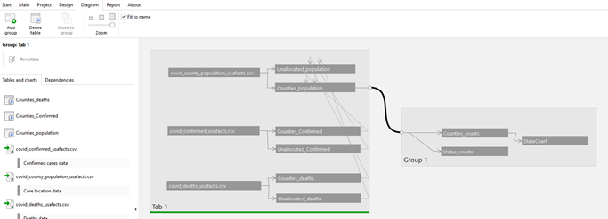
Selecting a group in the diagram will open a list of the datasets contained in that group in the left pane. Double-clicking a dataset in the diagram moves focus to that dataset in its group tab.
ADDING ACTIONS/TOOLS
In Alteryx, the primary method for adding tools to the canvas to build a workflow is pulling them down from the various toolbars at the top of the UI. Alternatively, right-clicking anywhere on the empty canvas space invokes a shortcut menu, allowing the user to insert any tool through the use of categorized submenus.
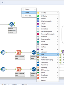
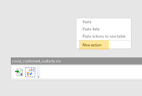
EasyMorph offers several ways to quickly add actions to the workflow. As with Alteryx, right-clicking the canvas area brings up a shortcut menu with the “New action” option. Selecting this opens the action selection list at the left of the UI.
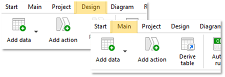
Additionally, the “Add action” button appears on both the Main and Design tabs in the ribbon at the top of the UI.
Selecting a dataset in the workflow, opens the left sidebar offering a list of the current actions in that dataset, along with the “Add new action” button.
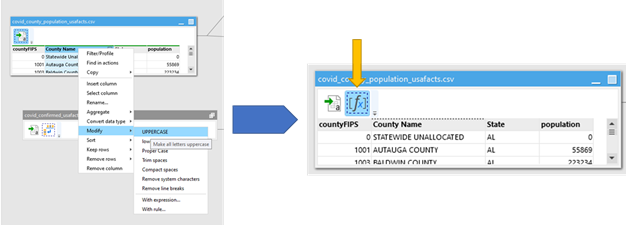
Finally, by either selecting the drop-down at the right of a data column’s heading, or right-clicking on the column’s heading, a context menu appears providing the user with a variety of options and transformations. Selecting an option from this list will create the corresponding action icon in the action row at the top of the dataset.
BRANCHING/SPLITTING DATASETS
In Alteryx, sending multiple copies of a dataset to downstream tools is done using multiple connectors from the output anchor of the current tool to the input anchors of the downstream receiving tools. As illustrated below, two copies of the datastream are send to both the Filter tool (top) and the Select tool (bottom).
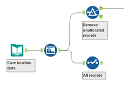
In EasyMorph, to split a dataset into two (or more) downstream branches, a copy of the source dataset is derived into multiple copies of itself. A derived table starts with the final form of the dataset, at the end of the workflow it is derived from.
Datasets in EasyMorph can also be Split at a specified point along the action row. Right-click on the action icon you wish to split at and select Split here . The dataset will be split into two. One instance keeps all actions from the start of the action chain to the action the split was initiated. This instance is now given a generic name (i.e., “Table 1”). The second instance keeps all actions that came after the action the split was initiated on. This instance keeps the original name of the dataset.
Subsequently, split tables can be re-merged by right-clicking the original, “pre-split” table (the table containing the initial actions in the chain, on the left, that received the generic table name) and selecting Merge derived table. In the example below, selecting the Merge derived table option on “Table 1” would append the actions in the “Counties_population” table to the end of the “Table 1” actions and rename the resultant table “Counties_population”.

JOINING/MERGING DATASETS
In Alteryx, when joining datasets together, Join tools will typically have two or more left input anchors to receive the datasets being joined. The user must properly connect the primary dataset to the correct anchor (typically the top anchor), and the secondary dataset to the bottom anchor. (Primary being the dataset being joined to, and the secondary being the dataset merging into. In some cases, a Join tool will have a single specialized, anchor that can accept multiple incoming datasets, i.e., the Join Multiple tool.)
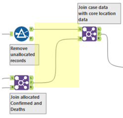
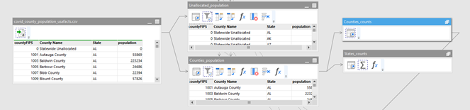
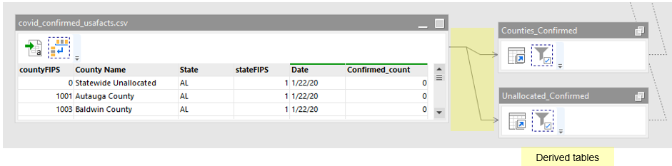
In EasyMorph, joining data happens as an action within the primary dataset using the Merge Another Table action. The matching columns to join on are selected in the action’s settings, and the columns from the reference table are defined. Dotted arrows leading from the reference table to the Merge Another Table action illustrate that data is being merged in. (Highlighted for reference in the image below, showing two datasets being merged into the primary dataset.)
The Merge Another Table action has three settings – defining the type of merge. Lookup acts much like the VLookup function in Excel. It matches each row in the primary dataset to one row in the reference dataset, ignoring all subsequent matches. The Left join setting matches all rows in the primary dataset to all matching rows in the reference dataset, creating duplicates of the primary records to match on all reference rows, if there is more than one match. The Full join setting creates a Cartesian product – outputting all records that match in both datasets, along with all records that do not have a match from both datasets.
Alteryx CONSTANTS, EasyMorph PARAMETERS
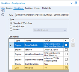
In Alteryx, if you need to reference a custom global value throughout your workflow, you create a constant. This is done in the Workflow – Configuration dialog by creating a label with an associated value. Constants, as the name implies, represent static values that do not change. By default, constant values are considered text unless the user selects the “#” checkbox, defining it as a number , instead.
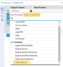
Constants can be used anywhere in the workflow where a value may be entered. For example (below), in a Formula tool, the constant can be called by referencing it similar to a field ( [square brackets] ), using the syntax “User.constant_name”. Constants can also be selected from the Columns and Constants list when building an expression.
EasyMorph’s parameter is the equivalent to the Alteryx’ constant – although it is capable of more than just representing static values.
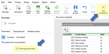
Parameters are set in the Edit Parameters window – accessed by either using the Edit Parameters button on the “Main” ribbon tab, or by clicking on the workflow canvas (the gray area between datasets) and using the button that appears in the “Overview” pane at the left.
You can define a parameter in EasyMorph as a text or number, a file name, a folder path, or a date. Parameters can be formulas referencing previously-defined parameters.
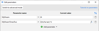
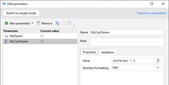
Switching the window to advanced mode will allow you to define additional settings for the parameter: a label (used in place of the defined Name), write notes, and even create validation rules.
The first role an EasyMorph parameter can take is that of representing a constant, unchanging value at the module level. This is the equivalent to Alteryx’s constant. These parameters are available anywhere within action settings where a downward arrow appears to the right of a setting box.
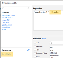
Parameters can be used in expressions by either typing out the parameter name in {curly braces} or selecting it from the Parameters list at the bottom-left corner of the Expression Editor.
The other role parameters can take on comes into play when calling other modules. Parameters are set up in the called module as “pathways” to receive incoming values from the calling module.
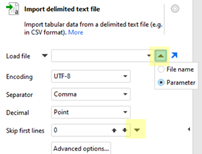
For example, when setting up an Iteration where a list of filenames is being passed to the called module, a parameter in the called module is set up through which the filenames are received. Multiple parameters can be defined within the called module to receive various pieces of data it may need to perform its process.
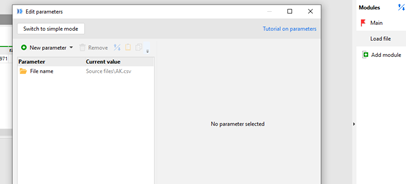
In this example, the "Main" module is passing in a list of filenames from a dataset to the "Load file" module. The "File name" parameter is created within the "Load file" module to receive the filenames from "Main".
ALTERYX MACRO EQUIVALENTS
In Alteryx, there are 3 types of macros. A macro is a self-contained workflow that is designed to receive data from an outside source (a calling workflow), process the data, and output the compiled data back out to the calling workflow. (The following descriptions and illustrations are overly simplified for the sake of clarity and are meant simply to pass along the concept of how each macro type works and the EasyMorph equivalent.)
STANDARD MACROS
Standard macros in Alteryx are simply workflows designed as simple pass-through processes and saved with a macro file extension. These macros take in one or more datasets, process them as designed, and pass the results back out to the calling workflow.
The EasyMorph equivalent would simply be a secondary module designed as a reusable workflow called from any other workflow/module.
BATCH MACROS
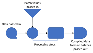
Alteryx batch macros are used to process data in batches, as the name implies, based on a set of values passed into the macro. A primary dataset is read in, along with the list of values that define the batch. Each value in the batch list is processed, applied to the primary dataset, until all values in the batch list have been consumed. The data compiled through all passes of the batch is then passed back out.
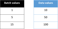
Example: A primary dataset contains numeric values. The batch dataset also contains numeric values to be multiplied to each of the values in the primary dataset. With each pass of the batch, the values in the primary dataset are multiplied by the current batch value, until all batch values have been processed. The macro then passes the compiled data from all batches out to the calling workflow. Given the tables below, the first batch would have a batch value of “1”. Each value in the dataset would be multiplied by “1”, and the end results would be held. Batch 2 multiplies the dataset values by “5”, and the results are appended to the results from the first batch and held. The third batch multiplies all dataset values by “15”, appends the results to the first two batches and, as this is the final batch value, the compiled results are passed out of the macro to the calling workflow.
In EasyMorph, the equivalent of this would be the Iterate action which repeatedly calls a second module, passing in a set of values via parameters to run through its process. The process runs until the set of values passed into the second module is exhausted. Results may be concatenated and returned to the calling dataset, or not returned at all if the purpose of the called module is to generate output (reports, emails, etc.), for example.
ITERATIVE MACROS
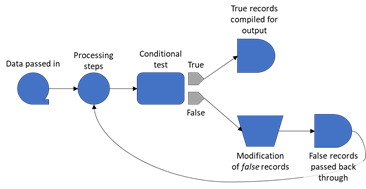
The third type of Alteryx macro is the iterative macro. With this type of macro, a dataset is passed in and processed. Towards the end of the macro, a T/F condition is set to branch the output. Records passing the condition are held. Any records failing the condition are altered in some way and looped back through the macro to be reprocessed. If any records now pass the condition, they are routed out the “true” branch while any records still failing are modified and looped back through again.
These macros are usually configured with a set number of loops before the macro stops processing and releases its results, or is constructed in such a way that eventually all records will pass the condition and be passed out.
In the first case, two datasets are passed out of the macro – the records that passed the condition, and those that did not pass the condition, if there are any.
In EasyMorph, the equivalent action would be the Repeat action that is designed to call a module repeatedly (up to a set maximum number of iterations to prevent endless loops), until a condition is met (UNTIL or WHILE the result table is empty).
ANALYTIC APPLICATIONS
Alteryx possesses another type of workflow called an Analytic Application, that really has no direct equivalent in EasyMorph. It is built as a standard workflow that includes a custom-built GUI the user can use to inject on-the-fly values into the workflow during runtime. It must be run using a special “Run as Analytic Application” button to function properly, otherwise it runs as a standard workflow.
Currently, EasyMorph doesn’t provide any run-time UI components to capture user input, although hopefully they’re on the roadmap for future release.
FLOW CONTROL
Alteryx uses two main tools, found under the Developer tab, to control the flow of a workflow.
Block Until Done takes a single data stream and provides 3 output anchors to connect downstream processes. Each output process is run through completion before the next branch starts (from top to bottom). This ensures sections of the workflow run in the order intended. Multiple Block Until Dones can be stacked to handle more than 3 downstream processes.
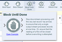
The EasyMorph equivalent would be the use of the Synchronize action to control the processing of individual datasets until other datasets’ actions are completed, and then continue.
Detour / Detour End allow a workflow to split into two possible processes, only one of which will actually run, based on the tool’s setting. A workflow branch is connected to each output anchor of the Detour tool (named “Left” and “Right”). The only setting in this tool is “Detour to the Right”, which is “off” by default, meaning the “left”/top process will fire. To change processing to the bottom (“right”) path, Developer tools are required to accept a boolean setting from another tool (or user input) and keep the setting “off”, or flip it “on” to divert to the “right”/bottom path.
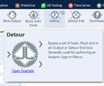
The closest equivalents in EasyMorph to Alteryx’s Detour/Detour End process would be the use of the Skip Actions on condition action, the Halt on condition action, or a pair derived tables at the point of the “detour”, set to opposing conditions (so only one of the derived tables processes).
DATA PROFILING
The primary tool in Alteryx for gaining insight into the data within a data stream is the Browse tool. Connecting a Browse to an output anchor provides the user with, A) the full output of the workflow to that point (instead of just the typical data sample), and B) statistics about each of the fields in the data stream. The Browse initially provides high level information about each field but selecting a specific field/column name will provide more in-depth information.
While it is suggested, and considered “standard practice”, to add a Browse tool anywhere in a workflow where data has drastically changed, the inclusion of Browse tools slows the workflow processing down as it generates all records of the dataset to that point. An overabundance of Browse tools can slow a workflow down to a crawl. The Browse tool has no output anchors and cannot pass its information along downstream.
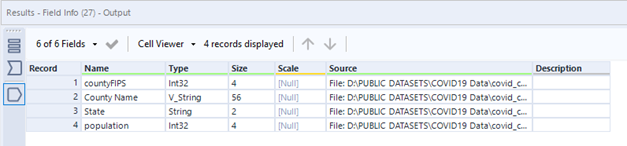
The other tool used to provide basic field information in the data stream is the Field Info tool found in the Developer tab. This tool, when connected to the output anchor of a tool will provide the name, data type, data size, scale, the original data source (file or connection), and description of each field in the dataset. The output anchor of the Field Info tool can be used to capture the field information downstream to use in processing or to print.
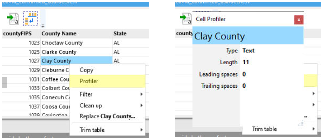
In EasyMorph, at the individual cell level within a dataset, cell metadata can be viewed by right-clicking any cell and selecting “Profiler” This opens a small window showing some specs of the selected cell. This window stays open so you can click around and explore other cells.
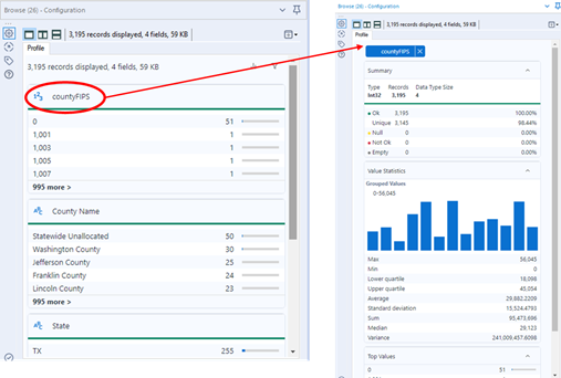
The next profiling “level up” is Column Profiling. The Column filter/profile window is activated by: 1) double-clicking a data column’s heading, 2) right-clicking a column’s heading and selecting “Filter/Profile”, or 3) clicking the down arrow at the right of a column’s heading and selecting “Filter/Profile”.
Within the Column Filter/Profile window, there are several tabs’ worth of details to be found: Values (value list and filter conditions), Profile (statistical details regarding the column’s data – types, counts, mins/maxes, lengths, etc.), Histogram (for numeric values), Suggestions (pointing out potential data quality issues), and Metadata (for the column as a whole). As with the cell profile window, this window remains open for you to select other columns to explore (click on another column or select another column from the top of the open window).
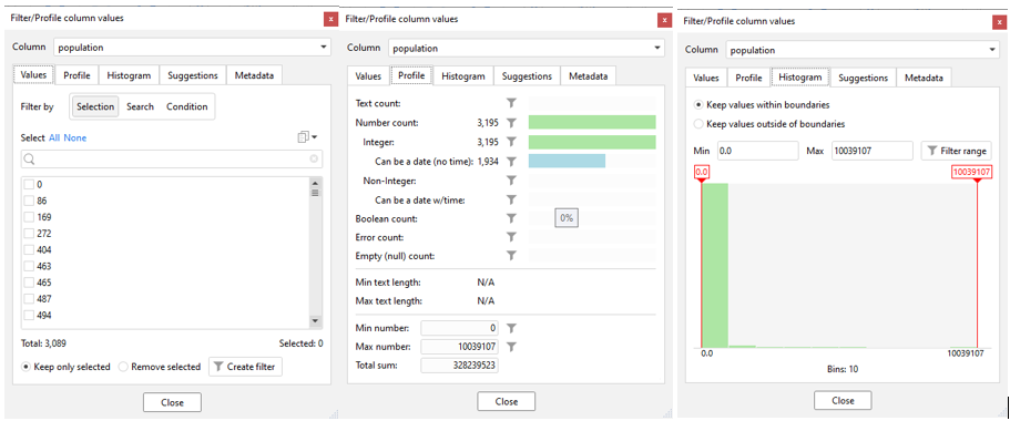
(The Values window, Profile window, and Historgram window for column profiling.)
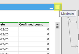
Finally, Analysis View shows top-level, table-wide statistics in a full-screen window. You can access this view by double-clicking a dataset’s title bar or clicking the Maximize button at the right end of the title bar.
The Analysis View window gives you “one-stop-shopping” for reviewing and filtering your dataset. By default, the window opens with the “filter pane” open on the top. You can drag columns into this area and set ad hoc filters across them.
Other options let you Search the dataset, Go to specific rows, and you can even step through and Add actions in this view.
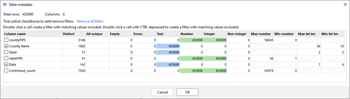
The Table metadata button opens a window displaying statistics for the table as a whole, with a column-by-column breakdown.
REPORTING OPTIONS
Alteryx boasts a pretty full-featured reporting process for turning data and insights into visuals to be printed or pdf’d, or formatted to be output to other applications (i.e., Excel). The concept for the reporting process is pretty simple. A set of Reporting tools accept specific datastream input – geospatial, data tables, text, etc. – and formats the datastream into a reporting object, or snippet . Text can become text blocks, header or footer text. Numeric data can be converted into formatted tables or charts. Geospatial data becomes formatted maps. Images become image snippets.
![]()
The Overlay tool allows for different snippets to be “stacked” or “laid over” one another in layers , while the layout tool assembles the different snippets together into the final report format by defining where each snippet appears (top/bottom, left/right) and how much space on the page each snippet occupies (in length or % of the page).
![]()
The final reporting step is the use of the Render tool, which takes all the information from the Layout tool and generates the final formatted output. An Email tool can be used to format auto-generated emails containing the report, or portions of the report, depending on where it is inserted in the workflow.

In comparison, at this time, EasyMorph has a more basic set of tools for laying out reports from its content using a more “Powerpoint-like” screen to hand-position the different elements on the page. Selecting the Report tab in the ribbon opens a report view of the objects in the active group. Along the left pane, table and chart objects can be selected/deselected to be shown or hidden on the report layout. Each table/chart displays as a free-floating object that can be positioned anywhere on the page.
Tables can be expanded or contracted – left/right, top/bottom – for the required view. Titles and annotations (footers) can be created for each object, and column totals can be defined for tables to show on the report – at the bottom of a dataset grid.
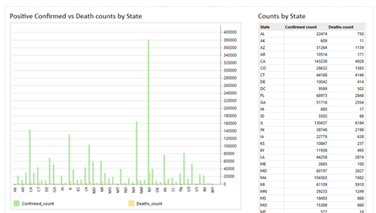
Similarly, chart objects can be resized and positioned where desired, with the only option for the legend being placed at the bottom or turned off completely.
Beyond the data-driven objects, clicking the Add layout item button on the Report ribbon allows the user to add formatted Text boxes, Paragraph boxes for longer formatted text, and Images.
Page Setup options (on the Report ribbon) include Paper size, orientation and margins (narrow/wide).
Given this, I would say the best way to handle reporting needs is to create a tab specific for report layout which would include only the tables and charts, in their final forms , that would be required for the report. Tables should be derived from the final stages of the datasets and renamed so they appear appropriately on the report (instead of a source filename showing in the title bar). Similarly, charts should be derived from the final aggregated form of data they are based on, and resized to show all graphics clearly.